View this project’s code on GitHub :)

Background

Melanoma

Melanoma is a deadly skin cancer. Out of all skin lesions,it is especially dangerous because it is outnumbered by other skin lesions, and it is difficult to identify. However, melanoma is best treated when caught early, so treatment relies on rapid identification.

According to the Skin Cancer Foundation, an estimated 7,180 people will die from melanoma in 2021 alone.

Machine Learning

Machine learning has been a successful tool for diagnosing other diseases from medical images. Many research groups have achieved high rates of accuracy, including algorithms outlined in the following papers:

• Mohammed et al., 2018
• Kang et al., 2017
• Lui & Kang, 2017

Machine learning algorithms have even already shown promise at the task of identifying melanoma. Hosny et al. (2019) achieved an accuracy of 95.91% on a dataset similar to that used in this research.

Almost all of these papers used some form of Convolutional Neural Network, or CNN, as it is generally considered the best algorithm for image recognition. CNNs are good at rapidly learning patterns in image data, making them a logical choice for this task.

However, a relatively new algorithm also shows significant promise at image recognition:

The QCNN

Note: for an explanation of quantum computing, see the Quantum Computing section in the Superdense Coding project.

The QCNN is a relatively new proposed structure for neural networks that takes advantage of quantum computing. As of the last time I checked, only one article has been published that uses a QCNN for image recognition, and no researchers have attempted to use if for melanoma identification thus far.

Structure

There are two main structures of quantum convolutional neural network, or QCNN:

• a combined classical / quantum network
• a purely quantum model

Both are similar in structure to a CNN.

The first replaces the first convolutional layer of a CNN with one or more quantum circuits. If more than one quantum circuit is used, the outputs are combined using a fully connected layer. The rest of the algorithm, however, is identical to a CNN.

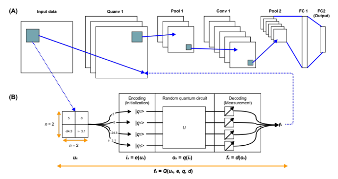
Image from Henderson et al., 2020

The second is entirely quantum, and is composed of a series of quantum circuits designed to replicate the functionality of the layers of a CNN.

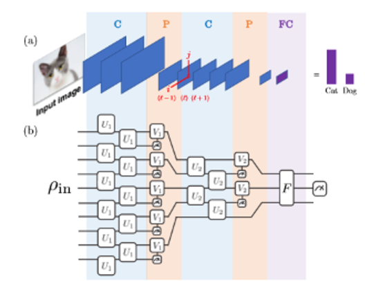
Image from Cong et al., 2019

The advantage of the QCNN is that theoretically, it can handle much larger data inputs and still process faster due to a much lower complexity than traditional models.

However, this isn’t currently the case. Modern quantum computers are still in development, and aren’t big enough to compete with classical ones yet.

The Image Size Problem

The largest quantum computer available through IBM is only 15 qubits, and since every pixel of a grey-scale input image would be one qubit, training on large input data is not feasible.

The solution to this problem employed in this research was to use the first QCNN structure. This allows the quantum circuit to be used much like a convolutional filter, sweeping over the image and only needing to compute with a couple inputs at a time.

Filter Circuits

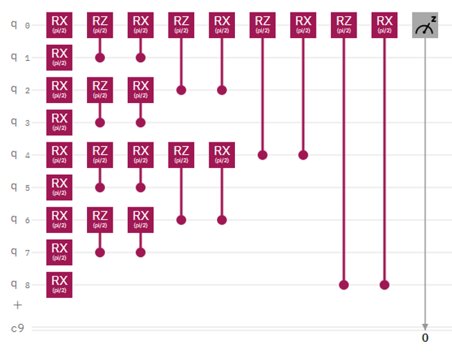
Image based on a design from Oh et al., 2020

This is a simplistic quantum filter circuit.

Each of the RX gates in the column on the left has a variable rotation, and together they act as an encoder. They allow classical values to be turned into quantum information by rotating a qubit an amount based on the classical value.

Each pair of controlled RZ and controlled RX gates acts as a pooling segment. The rotation of each gate is tunable, allowing the filter to be adjusted over the course of the learning process, and the fact that it has a control (marked by a small circle at the end of a line) on another qubit means that information is being mapped from all 9 initial qubits down to just one, which is measured at the end of the circuit.

This measurement returns a classical value which can then be used by the rest of the model.

The Quantum Advantage: Complexity

While the quantum computers of today cannot yet perform to their full theoretical potential, they still have a demonstrable advantage over classical computers in terms of complexity.

Image by me

The classical CNN filter has a complexity of O(n²). This means that the upper bound of the number of computations it performs grows as the square of the input size. In this case, the input size, n, is 3. This is the length of one side of the filter area. 9 computations are required for every element of the filter to be multiplied by the corresponding element of the image under the filter.

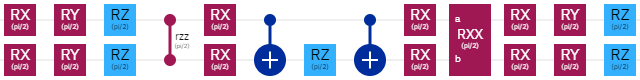
Image based on a design from Oh et al., 2020

The simple quantum filter circuit shown here has a complexity depth of O(⌈log₂(n²)⌉)*. This filter has an input size n of 2. The 2 by 2 area is flattened into a 4 by 1 matrix, which is input into the quantum circuit. The depth of the circuit is defined as the number of columns of gates. In this case, there are 6.

However, in complexity, we ignore both constants and numerical coefficients. Since the measurement column at the end and the encoder column at the beginning will both always be one depth, we disregard them. Additionally, each pooling segment will have a depth of 2, regardless of the input size, so we disregard that coefficient as well, leaving us with a complexity depth of 2 for an input size n of 2.

This aligns with the complexity depth of O(⌈log₂(n²)⌉), as 2² is 4, log₂(4) is 2, and ⌈2⌉ is 2.

*ceiling function denoted ⌈ ⌉

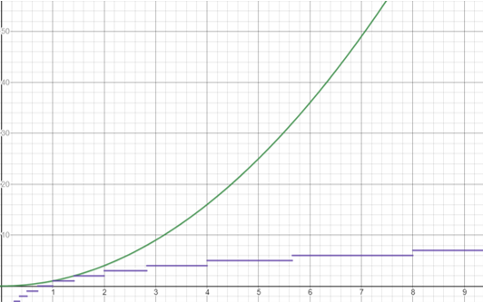
Image created by me, using Desmos

As you can see from the graphs of n² in green and ⌈log₂(n²)⌉ in purple, the complexity of the quantum filter grows much less quickly in relation to the input size than the classical filter does.

My Research

My goal over the course of my junior year was to create an adaptation of the first QCNN structure that could handle large image inputs. I planned to analyze the performance of the network on multiple test datasets, and compare it’s performance to the accuracies achieved by other networks, and the complexity of those networks.

The dataset I am using to train my network is the 512x512 combined melanoma dataset.

Quantum filter

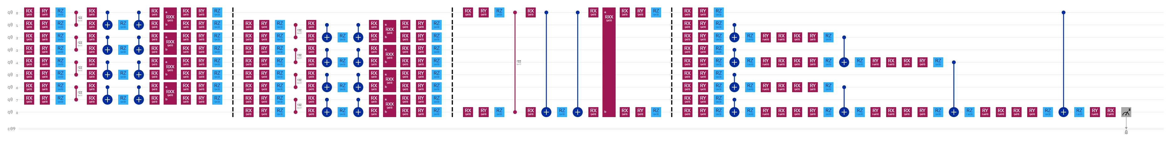
The quantum filter used in my network is more intricate than those shown previously, but it functions in much the same way.

Segment One

The first segment is an encoder. However, rather than encoding classical information by rotating only one qubit on its x axis, as the encoder of the simpler circuit did, it performs a rotation on two qubits simultaneously, and acts on all three axes of rotation.

Segment Two

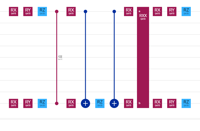
The second segment is also a part of the encoder, though it may look different. Each piece of the encoder looks like this: and encodes information onto two adjacent qubits. The first block of segment one encodes qubit pairs 0&1, 2&3, 4&5, and 6&7. The second block encodes pairs 1&2, 3&4, 5&6, and 7&8.

However, this only accounts for 8 of the 9 classical inputs, and only 8 of the 9 possible adjacent pairs. The final pair is 8&0. Segment two is simply the encoder piece for the 8&0 pair, and the final portion of the encoder.

Segment Three

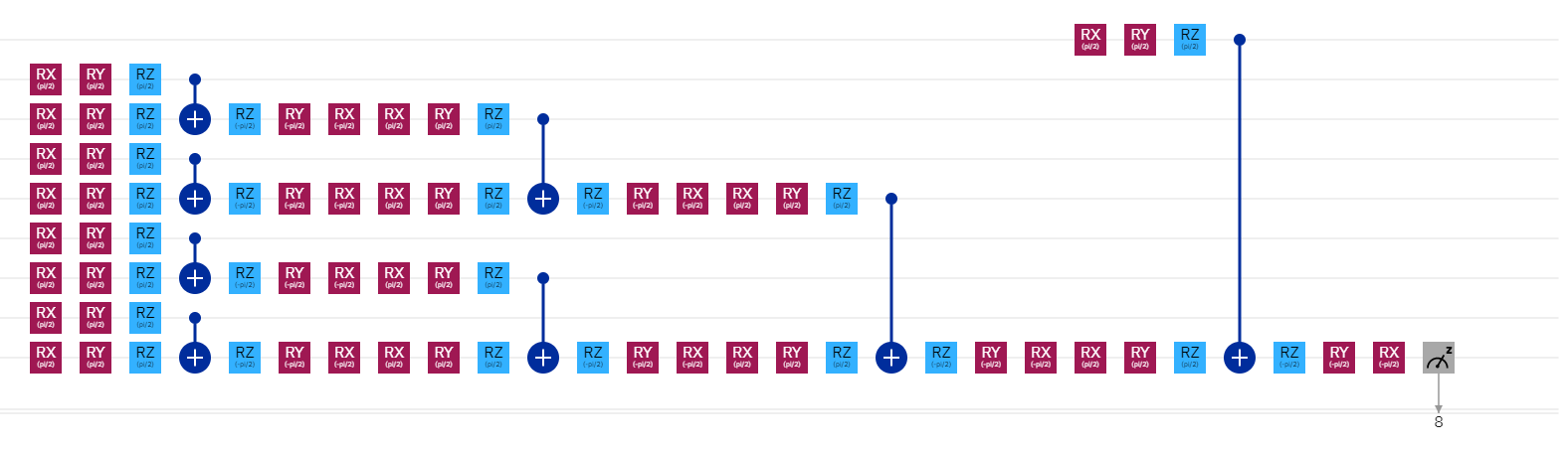
The third segment is the pooling segment. Like the encoder, it works much the same as the pooling segment of the simpler quantum circuit, but rather than just performing a rotation on the x and z axes, it uses rotations on all three axes, and a controlled not gate to pool the information.

The pooling segment combines the data from all of the qubits down to a single qubit, which is measured at the end of the circuit. The first column pools qubits 1-8 down to qubits 2, 4, 6, and 8. The second column pools those qubits to just 4 and 8. The thirds pools 4 and 8 to qubit 8, and the final column pools qubit 0 down to qubit 8 as well. Qubit 8 is then measured to obtain a single classical value as the result of the entire circuit.

Complexity

While it may seem like this filter circuit design would be far more complex than the simple filter circuit shown previously, it actually has the same complexity.

The encoding segment will always have either 34 or 51 depths. In the case of an input size of 3 (3x3 square, 9 total inputs), it will have 51. However, since this value alternates but will never increase beyond 51 as the input increases, it can be ignored in the complexity function.

The pooling segment also seem to have increased in complexity, but all that has changed is the depth of each section has gone from 2 to 7. We can represent the depth of each section of the pooling segment as L. For any given circuit, the value of L won’t change with a change in input size: only the number of sections required in the pooling segment will. Therefore, we can also remove the numerical coefficient L.

We are left with the same complexity depth as the simpler circuit: O(⌈log₂(n²)⌉)

Network Structure

I am using a tensorflow Keras sequential framework for my algorithm.

model = tf.keras.Sequential()

The first layer is my custom quantum layer.

model.add(qconv_64x64_trainable(image_to_circuit, add_pooling))

Next, there are 2 sets of two dimensional convolutional layers and two dimensional pooling layers.

model.add(tf.keras.layers.Conv2D(filters=32, kernel_size=3, activation='relu', input_shape=[61, 61]))
model.add(tf.keras.layers.MaxPool2D(pool_size=2, strides=2))
model.add(tf.keras.layers.Conv2D(filters=32, kernel_size=3, activation='relu'))
model.add(tf.keras.layers.MaxPool2D(pool_size=2, strides=2))

The data is then flattened.

model.add(tf.keras.layers.Flatten())

The network ends with a four-layer fully connected network with a binary output neuron.

model.add(tf.keras.layers.Dense(units=256, activation='relu'))
model.add(tf.keras.layers.Dense(units=256, activation='relu'))
model.add(tf.keras.layers.Dense(units=256, activation='relu'))
model.add(tf.keras.layers.Dense(units=256, activation='relu'))
model.add(tf.keras.layers.Dense(units=1, activation='sigmoid'))

The Custom Quantum Layer

This is the code for the custom quantum layer in my network:

class qconv_64x64_trainable (tf.keras.layers.Layer):
	def __init__(self, encoder, pooler):
        super(qconv_64x64_trainable, self).__init__()
        self.encode_data = encoder
        self.pool = pooler
        self.simulator = qsimcirq.QSimSimulator()

	def build(self, input_shape):
        self.kernel = self.add_weight("kernel", shape=[100,1])

	def call(self, input):
        tf.compat.v1.enable_eager_execution()
        print(tf.executing_eagerly())

        result = np.empty([61,61])
        for j in prange(0,input.shape[1]-3):
            for i in prange(0,input.shape[0]-3):
                print('input:',input,input.numpy())
                image_segment = input[0][j:j+4,i:i+4]
                iss_encoded_data = self.encode_data(image_segment)
                tbt_cirq_full = self.pool(iss_encoded_data, [self.kernel[i].numpy()[0] for i in range(90)])
                res = self.simulator.run(tbt_cirq_full).data.iat[0,0]
                result[j,i] = res
        return np.array([[result]])

Let’s go over it in a bit more detail.

The custom layer has three functions, based on the tensorflow Keras layer structure:

The init function

Almost all python classes have this function. This just sets up the object, and saves any constructor variables to the object.

def __init__(self, encoder, pooler):
	super(qconv_64x64_trainable, self).__init__()
	self.encode_data = encoder
	self.pool = pooler
	self.simulator = qsimcirq.QSimSimulator()

The first part of the __init__ function gets the superclass, which is the tensorflow Keras layer, and initializes it.

super(qconv_64x64_trainable, self).__init__()

Next, the variables passed when the object is initialized are stored. In this case, the variables encoder and pooler are stored to the object.

self.encode_data = encoder
self.pool = pooler

Finally, the simulator that will be used to compute the quantum circuit results is created. This uses the qsimcirq package, which is built for simulating large quantum circuits.

self.simulator = qsimcirq.QSimSimulator()

The build function

def build(self, input_shape):
	self.kernel = self.add_weight("kernel", shape=[100,1])

This one is a little simpler. The build function is called when the network is compiled, right before it is trained. It creates the layer’s kernel. This is the filter that passes over the image in a normal convolutional layer (see this gif). In the gif, the kernel has the shape [3,3]. However, in the custom layer, the kernel is initialized with the rather unusual shape [100,1], for reasons that will be explained in the next section.

The call function

def call(self, input):
	tf.compat.v1.enable_eager_execution()
	print(tf.executing_eagerly())

	result = np.empty([61,61])
	for j in range(0,input.shape[1]-3):
        for i in range(0,input.shape[0]-3):
            print('input:',input,input.numpy())
            image_segment = input[0][j:j+4,i:i+4]
            iss_encoded_data = self.encode_data(image_segment)
            tbt_cirq_full = self.pool(iss_encoded_data, [self.kernel[i].numpy()[0] for i in range(90)])
            res = self.simulator.run(tbt_cirq_full).data.iat[0,0]
            result[j,i] = res
	return np.array([[result]])

This is the big one. The call function is called every time an image passes through the layer. In a normal layer, it would be a fast, simple computation: the output would simply be the matrix multiplication of the input image and the kernel. However, this layer works a little differently.

First, we check to make sure that tensorflow is executing eagerly. This is because we want to be able to access the values of our tensors during this step, and we can only do this during eager execution. However, this doesn’t NOT need to be checked for every call, so this is an inefficiency in the current code.

tf.compat.v1.enable_eager_execution()
print(tf.executing_eagerly())

Next, we create an empty array to store our output in. Since we know that the input images will be scaled down to 64 by 64, and the size of the quantum kernel we will be using is 4 by 4, we know that the output will be 61 by 61, since there will be a strip of three pixels on the bottom and right edges of the input that the kernel cannot begin on, since some part of it would extend past the image.

result = np.empty([61,61])

These for loops loop through every pixel in the input image, besides those in the strips mentioned above.

for j in range(0,input.shape[1]-3):
	for i in range(0,input.shape[0]-3):

Within each for loop, we do a number of things.

print('input:',input,input.numpy())
image_segment = input[0][j:j+4,i:i+4]
iss_encoded_data = self.encode_data(image_segment)
tbt_cirq_full = self.pool(iss_encoded_data, [self.kernel[i].numpy()[0] for i in range(90)])
res = self.simulator.run(tbt_cirq_full).data.iat[0,0]
result[j,i] = res

1. Print the entire input, and the numpy array version of the input. This was another check for eager execution, as the numpy array would be inaccessible unless tensorflow were executing eagerly, but it should not be happening for every pixel.

2. Identify the segment of the of the image that the filter is looking at.

3. Encode the data. This is segments one and two of the filter circuit. The function that constructs this portion of the filter circuit is passed as the encoder in the __init__ function.

4. Construct the full circuit. This adds segment three to the circuit. The function that builds the pooling segment off of the encoder segment is passed as the pooler in the __init__ function.

   This is why we have such an oddly shaped kernel. Since, when the network is training, tensorflow automatically adjust the waits of the kernel, we are using the values of the kernel as the rotations for the adjustable gates in the quantum circuit. This way, the quantum circuit is automatically trained to work best with the dataset.

5. Simulate the circuit. This is done using the qsimcirq module.

6. Add the result of the circuit to the proper location in the output array.

Finally, outside the for loops, the array of results is returned and passed to the next portion of the network.

return np.array([[result]])

Results and Plans

Unfortunately, accuracy data could not be collected for the hybrid model that was designed in this research. The way the filter circuits are being implemented is incredibly inefficient. The entire circuit is built with different rotation values for the gates, then sent to a quantum computer and run, for every pixel of every image in the dataset. This makes training the network, even on an incredibly limited subset of the dataset, take such a long time as to render the algorithm useless.

Over the course of my senior year, this project will be revisited. I plan to rewrite much of the code, as well as work with experts in the quantum computing field to optimize the process by which I create the quantum circuits.

Sources

---